2 Analyzing Contingency Tables

table2_1 <- data.frame(Gender = c("Female", "Female", "Male", "Male"), 
                       Belief = c(" Yes", "No", " Yes", "No"),
                       Count = c(1230, 357, 859, 413))

addmargins(xtabs(Count ~ Gender + Belief, table2_1))

        Belief
Gender    Yes   No  Sum
  Female 1230  357 1587
  Male    859  413 1272
  Sum    2089  770 2859

2.1 Probability Structure for Contingency Tables

2.1.1 Joint, Marginal, and Conditional Probabilities

\[ \hat{\pi}_{ij} = n_{ij}/n \]

Sex	Yes	No or undecided
Females	\(\pi11\)	\(\pi12\)	\(\pi1+\)
Males	\(\pi21\)	\(\pi22\)	\(\pi2+\)
	\(\pi{{+}}1\)	\(\pi{{+}}2\)

\[ \pi_{1+} = \pi_{11} + \pi_{12}\ \ \mathrm{and}\ \ \pi_{+1} = \pi_{11} + \pi_{21} \] ### 2.1.2 Example: Sensitivity and Specificity

\[ \ \ \ \ \ \ \ \ \ \ \ \ \ \ \ \ \ \ \ \ \ \ prediction\ |\ truth \\ \mathrm{Sensitivity} = P(Y=1\ |\ X = 1), \\ \mathrm{Sepecificity} = P(Y=2\ |\ X = 2) \] ### 2.1.3 Statistical Independence of Two Categorical Variables

\[ P(X = i, Y = j) = P(X = i) P(Y = j)\ \mathrm{for}\ i = 1, ..., r\ \mathrm{and}\ j = 1,..., c. \]

2.1.4 Binomial and Multinomial Sampling

2.2 Comparing Proportions in 2 x 2 Contingency Tables

2.2.1 Difference of Proportions

\[ SE = \sqrt{\frac{\hat{\pi}_1 - (1 - \hat{\pi}_1)}{n_1} + \frac{\hat{\pi}_2 - (1 - \hat{\pi}_2)}{n_2}} \]

\[ (\hat{\pi}_1 - \hat{\pi}_2) \pm z_{\alpha/2}(SE) \]

2.2.2 Example: Aspirin and incidence of Heart Attacks

table2_2 <- tibble(Group = c("Placebo", "Placebo", "Aspirin", "Aspirin"), 
                       `Myocardial Infarction` = c(" Yes", "No", " Yes", "No"),
                       Count = c(189, 10845, 104, 10933))

addmargins(xtabs(Count ~ Group + `Myocardial Infarction`, table2_2))

         Myocardial Infarction
Group       Yes    No   Sum
  Aspirin   104 10933 11037
  Placebo   189 10845 11034
  Sum       293 21778 22071

\[ SE = \sqrt{\frac{(0.0171) (0.9829)}{11,034} + \frac{(0.0094) - (0.9906)}{11,0037}} = 0.0015 \]

2.2.3 Ratio of Proportions (Relative Risk)

\[\mathrm{Relative\ risk} = \frac{\pi_1}{\pi_2}\]

2.2.4 Using `R` for Comparing Proportions in 2 x 2 Tables

prop.test(c(189, 104), c(11034, 11037), correct = FALSE)


    2-sample test for equality of proportions without continuity correction

data:  c(189, 104) out of c(11034, 11037)
X-squared = 25.014, df = 1, p-value = 5.692e-07
alternative hypothesis: two.sided
95 percent confidence interval:
 0.004687751 0.010724297
sample estimates:
    prop 1     prop 2 
0.01712887 0.00942285

options(digits = 5)

library(PropCIs)
diffscoreci(189, 11034, 104, 11037, conf.level = 0.95)




data:  

95 percent confidence interval:
 0.0047168 0.0107885

riskscoreci(189, 11034, 104, 11037, conf.level = 0.95)




data:  

95 percent confidence interval:
 1.4339 2.3047

options(digits = 7)

2.3 The Odds Ratio

\[\mathrm{odds} = \pi/(1-\pi).\]

\[\pi = \mathrm{odds/(odds+1)}.\]

\[\theta =\frac{\mathrm{odds_1}}{\mathrm{odds_2}} = \frac{ \pi_1/(1-\pi_1)}{\pi_2/(1-\pi_2)},\]

2.3.1 Properties of the Odds Ratio

\[\theta=\frac{\pi_{11}/\pi_{12}}{\pi_{21}/\pi_{22}} = \frac{\pi_{11}\pi_{22}}{\pi_{12}\pi_{21}}.\]

\[\hat{\theta}=\frac{\hat{\pi}_1/(1-\hat{\pi}_1)}{\hat{\pi}_2/(1-\hat{\pi}_2)}=\frac{n_{11}/n_{12}}{n_{21}/n_{22}} = \frac{n_{11}n_{22}}{n_{12}n_{21}}.\]

2.3.2 Example: Odds Ratio for Aspirin and Hart Attacks

2.3.3 Inference for Odds Ratios and Log Odds Ratios

\[SE = \sqrt{\frac{1}{n_{11}}+ \frac{1}{n_{12}}+ \frac{1}{n_{21}}+\frac{1}{n_{22}}}.\]

\[log\ \hat{\theta} \pm z_{\alpha/2}(SE).\]

\[SE = \sqrt{\frac{1}{189}+ \frac{1}{10,933}+ \frac{1}{104}+\frac{1}{10,845}} = 0.123\] \[(\mathrm{exp}(0.365),\ \mathrm{exp}(0.846)) = (e^{0.365},\ e^{0.846}) = (1.44, 2.33).\]

library(epitools)
epitools::oddsratio(c(189, 10845, 104, 10933), method = "wald")

$data
          Outcome
Predictor  Disease1 Disease2 Total
  Exposed1      189    10845 11034
  Exposed2      104    10933 11037
  Total         293    21778 22071

$measure
          odds ratio with 95% C.I.
Predictor  estimate    lower   upper
  Exposed1 1.000000       NA      NA
  Exposed2 1.832054 1.440042 2.33078

$p.value
          two-sided
Predictor    midp.exact fisher.exact   chi.square
  Exposed1           NA           NA           NA
  Exposed2 4.989646e-07 5.032836e-07 5.691897e-07

$correction
[1] FALSE

attr(,"method")
[1] "Unconditional MLE & normal approximation (Wald) CI"

library(PropCIs)
# Score CI for odds ratio
orscoreci(189, 11034, 104, 11037, conf.level = 0.95)




data:  

95 percent confidence interval:
 1.440802 2.329551

2.3.4 Relationship Between Odds Ratio and Relative Risk

\[\mathrm{Odds\ ratio} = \frac{\hat{\pi}_1 / (1- \hat{\pi}_1)}{\hat{\pi}_2 / (1- \hat{\pi}_2)} = \mathrm{Relative\ risk} \times \left(\frac{1- \hat{\pi}_1}{1- \hat{\pi}_2} \right).\]

2.3.5 Example: The Odds Ratio Applies in Case-Control Studies

table2_3 <- data.frame(Smoker = c(" Yes", " Yes", "No", "No", "Total", "Total"), 
                       Belief = c(rep(c("Cases","Controls"),3)),
                       Count = c(688, 650, 21, 59, 709, 709))

xtabs(Count ~ Smoker + Belief, table2_3)

       Belief
Smoker  Cases Controls
   Yes    688      650
  No       21       59
  Total   709      709

\[\frac{(688/709)/(21/709)}{(650/709)/(59/709)} = \frac{688 \times 59}{650 \times 21} = 3.0.\]

2.3.6 Types of Studies Observational Versus Experimental

2.4 Chi-Squared Tests of Independence

2.4.1 Pearson Statistic and the Chi-Squared Distribution

\[\begin{equation} \chi^2= \sum\frac{(n_{ij}-\mu_{ij})^2}{\mu_{ij}}. \tag{2} \end{equation}\]

library(ggplot2)
library(ggthemes)
library(RColorBrewer)

colors <- brewer.pal(n = 4, name = "Dark2")

ggplot(data.frame(x = c(0, 40)), aes(x = x)) +
  stat_function(fun = dchisq, args = list(df = 1), color = colors[1]) +
  annotate(geom = "segment", x = 11, y = .11, xend = 2.2, yend = .11, 
    arrow = arrow(length = unit(2, "mm")), color = colors[1]) +
  annotate(geom = "text", x = 11.75, y = .11, label = "df = 1", 
           hjust = "left", color = colors[1]) +
  
  stat_function(fun = dchisq, args = list(df = 5), color = colors[2]) +
  annotate(geom = "segment", x = 11, y = .13, xend = 5, yend = .13, 
    arrow = arrow(length = unit(2, "mm")), color = colors[2]) +
  annotate(geom = "text", x = 11.75, y = .13, label = "df = 5", 
           hjust = "left", color = colors[2]) +
  
  stat_function(fun = dchisq, args = list(df = 10), color = colors[3]) +
  annotate(geom = "segment", x = 15, y = .08, xend = 11, yend = .08, 
    arrow = arrow(length = unit(2, "mm")), color = colors[3]) +
  annotate(geom = "text", x = 15.75, y = .08, label = "df = 10", 
           hjust = "left", color = colors[3]) + 
  
  stat_function(fun = dchisq, args = list(df = 20), color = colors[4]) +
  annotate(geom = "segment", x = 25, y = .055, xend = 22.5, yend = .055, 
    arrow = arrow(length = unit(2, "mm")), color = colors[4]) +
  annotate(geom = "text", x = 25.75, y = .055, label = "df = 20", 
           hjust = "left", color = colors[4]) + 
  ylim(c(0, 0.2)) +
  xlab("Chi-Squared") +
  ylab("Probability Denstiy") +
  theme_few()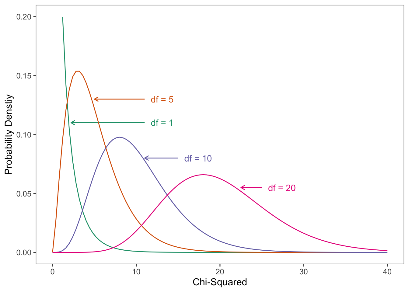

2.4.2 likelihood-Ratio Statistic

\[G^2 = 2\sum n_{ij}\ log \left(\frac{n_{ij}}{\mu_{ij}}\right).\]

2.4.3 Testing Independence in Two-Way Contingency Tables

\[H_0: \pi_{ij} = \pi_{i+} \pi_{+j}\ \mathrm{for\ all}\ i\ \mathrm{and}\ j.\]

\[\hat\mu_{ij}= n\hat\pi_{i+}\hat\pi_{+j}= n \left(\frac{n_{i+}}{n}\right) \left(\frac{n_{+j}}{n}\right) = \frac{n_{i+}n_{+j}}{n}\]

\[df=(rc-1)-[(r-1) + (c-1)] = rc -r -c +1 = (r-1)(c-1)\]

2.4.4 Example: Gender Gap in Political Party Affiliation

Political <- read.table("http://users.stat.ufl.edu/~aa/cat/data/Political.dat",
                        header = TRUE)

Political <- Political %>% 
  mutate(Party = factor(party, levels = c("Dem", "Rep", "Ind")))

library(gmodels)
CrossTable(Political$gender, Political$Party, expected = TRUE, prop.c = FALSE,
           prop.r = FALSE, prop.t = FALSE, prop.chisq=FALSE)


 
   Cell Contents
|-------------------------|
|                       N |
|              Expected N |
|-------------------------|

 
Total Observations in Table:  2450 

 
                 | Political$Party 
Political$gender |       Dem |       Rep |       Ind | Row Total | 
-----------------|-----------|-----------|-----------|-----------|
          female |       495 |       272 |       590 |      1357 | 
                 |   456.949 |   297.432 |   602.619 |           | 
-----------------|-----------|-----------|-----------|-----------|
            male |       330 |       265 |       498 |      1093 | 
                 |   368.051 |   239.568 |   485.381 |           | 
-----------------|-----------|-----------|-----------|-----------|
    Column Total |       825 |       537 |      1088 |      2450 | 
-----------------|-----------|-----------|-----------|-----------|

 
Statistics for All Table Factors


Pearson's Chi-squared test 
------------------------------------------------------------
Chi^2 =  12.56926     d.f. =  2     p =  0.00186475

2.4.5 Residuals for Cells in a Contingency Table

\[\frac{n_{ij} - \hat\mu_{ij}} {\sqrt{\hat\mu_{ij}(1-\hat\pi_{i+})(1-\hat\pi_{+j})}} = \frac{n(\hat\pi_{ij} - {\hat\pi_{i+}\hat\pi_{+j})}} {\sqrt{n\hat\pi_{i+}\hat\pi_{+j}(1-\hat\pi_{i+})(1-\hat\pi_{+j})}}\]

Political <- read.table("http://users.stat.ufl.edu/~aa/cat/data/Political.dat",
                        header = TRUE)

# Political <- Political %>% 
#  mutate(party = factor(party, levels = c("Dem", "Rep", "Ind"))) %>% 
#  filter(party != "Ind")

library(gmodels)
CrossTable(Political$gender, Political$party, prop.r=FALSE, prop.c=FALSE,
           prop.t=FALSE, prop.chisq=FALSE, sresid=TRUE, asresid=TRUE)


 
   Cell Contents
|-------------------------|
|                       N |
|-------------------------|

 
Total Observations in Table:  2450 

 
                 | Political$party 
Political$gender |       Dem |       Ind |       Rep | Row Total | 
-----------------|-----------|-----------|-----------|-----------|
          female |       495 |       590 |       272 |      1357 | 
-----------------|-----------|-----------|-----------|-----------|
            male |       330 |       498 |       265 |      1093 | 
-----------------|-----------|-----------|-----------|-----------|
    Column Total |       825 |      1088 |       537 |      2450 | 
-----------------|-----------|-----------|-----------|-----------|

Political %>% 
  filter(row_number() %in% c(1, 2, n()))

  person gender party
1      1 female   Dem
2      2 female   Dem
3   2450   male   Ind

GenderGap <- 
  xtabs(~gender + party, data = Political)

chisq.test(GenderGap)


    Pearson's Chi-squared test

data:  GenderGap
X-squared = 12.569, df = 2, p-value = 0.001865

stdres <- chisq.test(GenderGap)$stdres
stdres

        party
gender         Dem       Ind       Rep
  female  3.272365 -1.032199 -2.498557
  male   -3.272365  1.032199  2.498557

library(vcd)

Loading required package: grid

conflict_prefer("oddsratio", "vcd")

[conflicted] Will prefer vcd::oddsratio over any other package.

mosaic(GenderGap, gp=shading_Friendly, residuals = stdres,
       residuals_type="Std\nresiduals", labeling = labeling_residuals())

2.4.6 Partitioning Chi-Squared Statistics

2.4.7 Limitations of Chi-Squared Tests

2.5 Testing Independence for Ordinal Variables

2.5.1 Linear Trend Alternative to Independence

\[R = \frac{\sum_{i,j}(u_i-\bar{u})(v_j-\bar{v})\hat\pi_{ij}} {\sqrt{\left[\sum_i(u_i-\bar{u})^2 \hat\pi_{i+}\right]{\left[\sum_j(v_i-\bar{v})^2 \hat\pi_{+j}\right]}}} \]

\[M^2 = (n-1)R^2\]

2.5.2 Example: Alcohol Use and Infant Malformation

Malform <- matrix(c(17066, 14464, 788, 126, 37, 48, 38, 5, 1, 1), ncol = 2)
`Table 2.6` <-  bind_cols(Alcohol = c("0", "<1", "1-2", "3-5", ">5"),
                     as.data.frame(Malform)) %>% 
  rename("Abscent" = V1, "Present" = V2) %>% 
  mutate(Total = Abscent + Present) %>% 
  mutate(Percent = round(Present / Total * 100, 2))

`Table 2.6`

  Alcohol Abscent Present Total Percent
1       0   17066      48 17114    0.28
2      <1   14464      38 14502    0.26
3     1-2     788       5   793    0.63
4     3-5     126       1   127    0.79
5      >5      37       1    38    2.63

Malform <- matrix(c(17066, 14464, 788, 126, 37, 48, 38, 5, 1, 1), ncol = 2)
Malform

      [,1] [,2]
[1,] 17066   48
[2,] 14464   38
[3,]   788    5
[4,]   126    1
[5,]    37    1

library(vcdExtra)

Loading required package: gnm

CMHtest(Malform, rscores = c(0, .5, 1.5, 4, 7), overall = TRUE)

Cochran-Mantel-Haenszel Statistics 

                 AltHypothesis   Chisq Df     Prob
cor        Nonzero correlation  6.5699  1 0.010372
rmeans  Row mean scores differ 12.0817  4 0.016754
cmeans  Col mean scores differ  6.5699  1 0.010372
general    General association 12.0817  4 0.016754

sqrt(6.5699)

[1] 2.563182

1 - pnorm(sqrt(6.5699))

[1] 0.005185889

2.5.3 Ordinal Tests Usually Have Greater Power

2.5.4 Choice of Scores

2.5.6 Trend Tests for r x 2 and 2 x c and Nominal-Ordinal Tables

2.6 Exact Frequentist and Bayesian Inference

2.6.1 Fisher’s Exact Test for 2 x 2 Tables

2.6.2 Example: Fisher’s Tea Tasting Colleague

tea <- matrix(c(3,1,1,3), ncol = 2)
fisher.test(tea)


    Fisher's Exact Test for Count Data

data:  tea
p-value = 0.4857
alternative hypothesis: true odds ratio is not equal to 1
95 percent confidence interval:
   0.2117329 621.9337505
sample estimates:
odds ratio 
  6.408309

fisher.test(tea, alternative = "greater")


    Fisher's Exact Test for Count Data

data:  tea
p-value = 0.2429
alternative hypothesis: true odds ratio is greater than 1
95 percent confidence interval:
 0.3135693       Inf
sample estimates:
odds ratio 
  6.408309

2.6.3 Conservatism for Actual P(Type I Error); Mid P-Value

library(epitools)
ormidp.test(3,1,1,3, or = 1)

  one.sided two.sided
1 0.1285714 0.2571429

2.6.4 Small-Sample Confidence Intervals for Odds Ratio

library(epitools)
or.midp(c(3,1,1,3), conf.level = 0.95)$conf.int

[1]   0.3100508 306.6338538

2.6.5 Bayesian Estimation for Association Measures

2.6.6 Example: Bayesian Inference in a Small Clinical Trial

library(PropCIs)
orci.bayes(11, 11, 0, 1, 0.5, 0.5, 0.5, 0.5, 0.95, nsim = 1000000)

[1] 3.276438e+00 1.361274e+06

diffci.bayes(11, 11, 0, 1, 0.5, 0.5, 0.5, 0.5, 0.95, nsim = 1000000)

[1] 0.09899729 0.99327276

pi1 <- rbeta(100000000, 11.5, 0.5)
pi2 <- rbeta(100000000, 0.5, 1.5)

options(scipen=99)  # default was 0
or <- pi1*(1-pi2)/((1-pi1) * pi2)
quantile(or, c(0.025, 0.975))

quantile(pi1 - pi2, c(0.025, 0.975))
mean(pi1 < pi2)

2.7 Association in Three-Way Tables

2.7.1 Partial Tables

2.7.2 Example: Death Penalty Verdicts and Race

death <- matrix(c(53, 414, 11.3, 
                  11, 37, 22.9,
                  0, 16, 0,
                  4, 139, 2.8,
                  53, 430, 11,
                  15, 176, 7.9), ncol = 3, byrow = TRUE)


`Table 2.9` <-  bind_cols(`Victims' Race` = c("White", "", "Black", "", "Total",  ""),
  `Defendants' Race` = rep(c("White", "Black"),3),
                     as.data.frame(death)) %>% 
  mutate(Total = V1 + V2) %>% 
  rename("Got Death Penalty" = V1, "Not Death Penalty" = V2, "Percent Yes" = V3) 
  

`Table 2.9`

  Victims' Race Defendants' Race Got Death Penalty Not Death Penalty
1         White            White                53               414
2                          Black                11                37
3         Black            White                 0                16
4                          Black                 4               139
5         Total            White                53               430
6                          Black                15               176
  Percent Yes Total
1        11.3   467
2        22.9    48
3         0.0    16
4         2.8   143
5        11.0   483
6         7.9   191

# race association victim and defendant OR
round((467 * 143 )/(48 * 16), 0)

[1] 87

# victim race by death penalty - whites
53 + 11

[1] 64

414 + 37

[1] 451

# victim race by death penalty - blacks
0 + 4

[1] 4

16 + 139

[1] 155

# odds DP for white victim
(53 + 11) / (414 + 37)

[1] 0.1419069

# odds DP for black victim 
(4 / (16 + 139))

[1] 0.02580645

# OR of DP for white victim relative to black   
((53 + 11) / (414 + 37)) / (4 / (16 + 139))

[1] 5.498891