5 Building and Applying Logistic Regression Models
5.1 Strategies in Model Selection
5.1.2 Example: Horseshoe Crab Satellites Revisited
\[\mathrm{logit}[P(Y=1)] = \alpha + \beta_1 weight + \beta_2 width + \beta_3 c_2 + \beta_4 c_3 + \beta_5 c_4 + \beta_6 s_2 + \beta_7 s_3\]
Crabs <- read.table("http://users.stat.ufl.edu/~aa/cat/data/Crabs.dat",
  header = TRUE, stringsAsFactors = TRUE
)

fit <- glm(y ~ weight + width + factor(color) + factor(spine),
  family = binomial, data = Crabs
)

summary(fit)
Call:
glm(formula = y ~ weight + width + factor(color) + factor(spine),
    family = binomial, data = Crabs)

Deviance Residuals:
    Min       1Q   Median       3Q      Max
-2.1977  -0.9424   0.4849   0.8491   2.1198

Coefficients:
               Estimate Std. Error z value Pr(>|z|)
(Intercept)    -8.06501    3.92855  -2.053   0.0401 *
weight          0.82578    0.70383   1.173   0.2407
width           0.26313    0.19530   1.347   0.1779
factor(color)2 -0.10290    0.78259  -0.131   0.8954
factor(color)3 -0.48886    0.85312  -0.573   0.5666
factor(color)4 -1.60867    0.93553  -1.720   0.0855 .
factor(spine)2 -0.09598    0.70337  -0.136   0.8915
factor(spine)3  0.40029    0.50270   0.796   0.4259
---
Signif. codes:  0 '***' 0.001 '**' 0.01 '*' 0.05 '.' 0.1 ' ' 1

(Dispersion parameter for binomial family taken to be 1)

    Null deviance: 225.76  on 172  degrees of freedom
Residual deviance: 185.20  on 165  degrees of freedom
AIC: 201.2

Number of Fisher Scoring iterations: 4
pValue <- 1 - pchisq(225.76 - 185.20, 172 - 165)
format(round(pValue, 8), scientific = FALSE)[1] "0.00000098"library(car)
Anova(fit)Analysis of Deviance Table (Type II tests)
Response: y
LR Chisq Df Pr(>Chisq)
weight 1.4099 1 0.23507
width 1.7968 1 0.18010
factor(color) 7.5958 3 0.05515 .
factor(spine) 1.0091 2 0.60377
---
Signif. codes: 0 '***' 0.001 '**' 0.01 '*' 0.05 '.' 0.1 ' ' 15.1.6 AIC and the Bias/Variance Tradeoff
\[\mathrm{AIC = -2(log\ likelihood) + 2(number\ of\ parameters\ in\ model).}\]
Crabs <- read.table("http://users.stat.ufl.edu/~aa/cat/data/Crabs.dat",
  header = TRUE, stringsAsFactors = TRUE
)

fit <- glm(y ~ width + factor(color), family = binomial, data = Crabs)

-2*logLik(fit)
'log Lik.' 187.457 (df=5)AIC(fit) # adds 2(number of parameters) = 2(5) = 10 to -2*logLik(fit)[1] 197.457fit <- glm(y ~ width + factor(color) + factor(spine),
family = binomial, data = Crabs)
library(MASS)
stepAIC(fit)Start: AIC=200.61
y ~ width + factor(color) + factor(spine)
Df Deviance AIC
- factor(spine) 2 187.46 197.46
<none> 186.61 200.61
- factor(color) 3 194.43 202.43
- width 1 208.83 220.83
Step: AIC=197.46
y ~ width + factor(color)
Df Deviance AIC
<none> 187.46 197.46
- factor(color) 3 194.45 198.45
- width 1 212.06 220.06
Call:  glm(formula = y ~ width + factor(color), family = binomial, data = Crabs)

Coefficients:
   (Intercept)           width  factor(color)2  factor(color)3  factor(color)4
     -11.38519         0.46796         0.07242        -0.22380        -1.32992

Degrees of Freedom: 172 Total (i.e. Null);  168 Residual
Null Deviance:      225.8
Residual Deviance: 187.5 AIC: 197.5library(tidyverse)
# need response variable in last column of data file
Crabs2 <- Crabs %>%
select(weight, width, color, spine, y)
library(leaps)
library(bestglm)
bestglm(Crabs2, family = binomial, IC = "AIC") # can also use IC="BIC"Morgan-Tatar search since family is non-gaussian.AIC
BICq equivalent for q in (0.477740316103793, 0.876695783647898)
Best Model:
Estimate Std. Error z value Pr(>|z|)
(Intercept) -10.0708390 2.8068339 -3.587971 3.332611e-04
width 0.4583097 0.1040181 4.406056 1.052696e-05
color -0.5090467 0.2236817 -2.275763 2.286018e-025.2 Model Checking
5.2.1 Goodness of Fit: Model Comparison Using the Deviance
\[G^2 = 2\sum\mathrm{observed[log(observed/fitted)]}\]
5.2.2 Example: Goodness of Fit for Marijuana Use Survey
library(tidyverse)
Marijuana <- read.table("http://users.stat.ufl.edu/~aa/cat/data/Marijuana.dat",
                        header = TRUE, stringsAsFactors = TRUE)
Marijuana
race gender yes no
1 white female 420 620
2 white male 483 579
3 other female 25 55
4 other male 32 62fit <- glm(yes/(yes+no) ~ gender + race, weights = yes + no, family = binomial,
data = Marijuana)
summary(fit) # deviance info is extracted on the next two lines
Call:
glm(formula = yes/(yes + no) ~ gender + race, family = binomial,
    data = Marijuana, weights = yes + no)

Deviance Residuals:
       1         2         3         4
-0.04513   0.04402   0.17321  -0.15493

Coefficients:
            Estimate Std. Error z value Pr(>|z|)
(Intercept) -0.83035    0.16854  -4.927 8.37e-07 ***
gendermale   0.20261    0.08519   2.378  0.01739 *
racewhite    0.44374    0.16766   2.647  0.00813 **
---
Signif. codes:  0 '***' 0.001 '**' 0.01 '*' 0.05 '.' 0.1 ' ' 1

(Dispersion parameter for binomial family taken to be 1)

    Null deviance: 12.752784  on 3  degrees of freedom
Residual deviance:  0.057982  on 1  degrees of freedom
AIC: 30.414

Number of Fisher Scoring iterations: 3fit$deviance # deviance goodness-of-fit statistic[1] 0.05798151fit$df.residual # residual df[1] 11 - pchisq(fit$deviance, fit$df.residual )[1] 0.8097152fitted(fit) 1 2 3 4
0.4045330 0.4541297 0.3035713 0.3480244 library(dplyr)
Marijuana %>%
mutate(fit.yes = (yes+no)*fitted(fit)) %>%
mutate(fit.no = (yes+no)*(1-fitted(fit))) %>%
select(race, gender, yes, fit.yes, no, fit.no) race gender yes fit.yes no fit.no
1 white female 420 420.71429 620 619.28571
2 white male 483 482.28571 579 579.71429
3 other female 25 24.28571 55 55.71429
4 other male 32 32.71429 62 61.285715.2.4 Residuals for Logistic Models with Categorical Predictors
\[\mathrm{Standardized\ residual} = \frac{y_i-n_i\hat\pi_i}{SE}.\] ### 5.2.5 Example: Graduate Admissoins at University of Florida
library(tidyverse)
Admissions <- read.table("http://users.stat.ufl.edu/~aa/cat/data/Admissions.dat",
                        header = TRUE, stringsAsFactors = TRUE)

theModel <- glm(yes/(yes+no) ~ department, family = binomial,
                data = Admissions,
                weights = yes+no)

theResiduals <- tibble(`Std. Res.` = rstandard(theModel, type = "pearson")) %>%
  mutate(`Std. Res.` = round(`Std. Res.`, 2)) %>%
  dplyr::filter(row_number() %% 2 == 0)  # every other record is female


theTable <- Admissions %>%
  mutate(gender = case_when(gender == 1 ~ "Female",
                            gender == 0 ~ "Male")) %>%
  pivot_wider(id_cols = department, names_from = gender,
              values_from = c(yes, no), names_sep = "") %>%
  select(department, yesFemale, noFemale, yesMale, noMale) %>%
  rename("Dept" = department, "Females (Yes)" = yesFemale, "Females (No)" =
           noFemale, "Males (Yes)" = yesMale, "Males (No)" = noMale) %>%
  bind_cols(theResiduals)

knitr::kable(theTable)| Dept | Females (Yes) | Females (No) | Males (Yes) | Males (No) | Std. Res. |
|---|---|---|---|---|---|
| anthropol | 32 | 81 | 21 | 41 | -0.76 |
| astronomy | 6 | 0 | 3 | 8 | 2.87 |
| chemistry | 12 | 43 | 34 | 110 | -0.27 |
| classics | 3 | 1 | 4 | 0 | -1.07 |
| communicat | 52 | 149 | 5 | 10 | -0.63 |
| computersci | 8 | 7 | 6 | 12 | 1.16 |
| english | 35 | 100 | 30 | 112 | 0.94 |
| geography | 9 | 1 | 11 | 11 | 2.17 |
| geology | 6 | 3 | 15 | 6 | -0.26 |
| germanic | 17 | 0 | 4 | 1 | 1.89 |
| history | 9 | 9 | 21 | 19 | -0.18 |
| latinamer | 26 | 7 | 25 | 16 | 1.65 |
| linguistics | 21 | 10 | 7 | 8 | 1.37 |
| mathematics | 25 | 18 | 31 | 37 | 1.29 |
| philosophy | 3 | 0 | 9 | 6 | 1.34 |
| physics | 10 | 11 | 25 | 53 | 1.32 |
| polisci | 25 | 34 | 39 | 49 | -0.23 |
| psychology | 2 | 123 | 4 | 41 | -2.27 |
| religion | 3 | 3 | 0 | 2 | 1.26 |
| romancelang | 29 | 13 | 6 | 3 | 0.14 |
| sociology | 16 | 33 | 7 | 17 | 0.30 |
| statistics | 23 | 9 | 36 | 14 | -0.01 |
| zoology | 4 | 62 | 10 | 54 | -1.76 |
\[logit(\pi_{ik}) = \alpha + \beta_k.\]
5.2.6 Standardized versus Pearson and Deviance Residuals
fit <- glm(yes/(yes+no) ~ gender + race, weights = yes + no, family = binomial,
           data = Marijuana)

summary(fit)
Call:
glm(formula = yes/(yes + no) ~ gender + race, family = binomial,
    data = Marijuana, weights = yes + no)

Deviance Residuals:
       1         2         3         4
-0.04513   0.04402   0.17321  -0.15493

Coefficients:
            Estimate Std. Error z value Pr(>|z|)
(Intercept) -0.83035    0.16854  -4.927 8.37e-07 ***
gendermale   0.20261    0.08519   2.378  0.01739 *
racewhite    0.44374    0.16766   2.647  0.00813 **
---
Signif. codes:  0 '***' 0.001 '**' 0.01 '*' 0.05 '.' 0.1 ' ' 1

(Dispersion parameter for binomial family taken to be 1)

    Null deviance: 12.752784  on 3  degrees of freedom
Residual deviance:  0.057982  on 1  degrees of freedom
AIC: 30.414

Number of Fisher Scoring iterations: 3knitr::kable(
bind_cols(Standardized = rstandard(fit, type = "pearson"),
Pearson = residuals(fit, type = "pearson"),
deviance = residuals(fit, type = "deviance"),
`std dev.` = rstandard(fit, type = "deviance"),
Race = Marijuana$race, Gender = Marijuana$gender) %>%
mutate_if(is.numeric, round, digits = 3)
)| Standardized | Pearson | deviance | std dev. | Race | Gender |
|---|---|---|---|---|---|
| -0.241 | -0.045 | -0.045 | -0.241 | white | female |
| 0.241 | 0.044 | 0.044 | 0.241 | white | male |
| 0.241 | 0.174 | 0.173 | 0.240 | other | female |
| -0.241 | -0.155 | -0.155 | -0.241 | other | male |
5.2.8 Example: Heart Disease and Blood Pressure
HeartBP <- read.table("http://users.stat.ufl.edu/~aa/cat/data/HeartBP.dat",
                      header = TRUE, stringsAsFactors = TRUE)

theModel <- glm(y/n ~ bp, family = binomial, data = HeartBP, weights = n)
summary(theModel)
Call:
glm(formula = y/n ~ bp, family = binomial, data = HeartBP, weights = n)

Deviance Residuals:
    Min       1Q   Median       3Q      Max
-1.0617  -0.5977  -0.2245   0.2140   1.8501

Coefficients:
             Estimate Std. Error z value Pr(>|z|)
(Intercept) -6.082033   0.724320  -8.397  < 2e-16 ***
bp           0.024338   0.004843   5.025 5.03e-07 ***
---
Signif. codes:  0 '***' 0.001 '**' 0.01 '*' 0.05 '.' 0.1 ' ' 1

(Dispersion parameter for binomial family taken to be 1)

    Null deviance: 30.0226  on 7  degrees of freedom
Residual deviance:  5.9092  on 6  degrees of freedom
AIC: 42.61

Number of Fisher Scoring iterations: 4
predicted <- round(fitted(theModel)* HeartBP$n, 1)
std_res <- round(rstandard(theModel, type = "pearson"),2)
#influence.measures(theModel)
rDfbeta <- data.frame(dfbetas(theModel)) %>%
select(bp) %>%
transmute(DFbeta = round(bp, 2))
HeartBP %>%
rename("Blood Presure" = bp,
"Sample size" = n,
"Observed Disease" = y) %>%
bind_cols("Fitted Disease" = predicted,
"Standardized Residual" = std_res,
"Dfbeta (not SAS)" = rDfbeta) Blood Presure Sample size Observed Disease Fitted Disease
1 111.5 156 3 5.2
2 121.5 252 17 10.6
3 131.5 284 12 15.1
4 141.5 271 16 18.1
5 151.5 139 12 11.6
6 161.5 85 8 8.9
7 176.5 99 16 14.2
8 191.5 43 8 8.4
Standardized Residual DFbeta
1 -1.11 0.56
2 2.37 -2.24
3 -0.95 0.34
4 -0.57 0.08
5 0.13 0.01
6 -0.33 -0.06
7 0.65 0.38
8 -0.18 -0.11library(ggthemes)
predicted <- predict(theModel, type = "response")
HeartBP %>%
mutate(proportion=y/n) %>%
ggplot(aes(x= bp, y = proportion)) +
geom_point(shape = 4) +
geom_smooth(aes(y = predicted)) +
theme_few() +
scale_x_continuous(breaks = seq(110, 200, by = 10), limits = c(110, 200)) +
ggtitle("Figure 5.1")`geom_smooth()` using method = 'loess' and formula = 'y ~ x'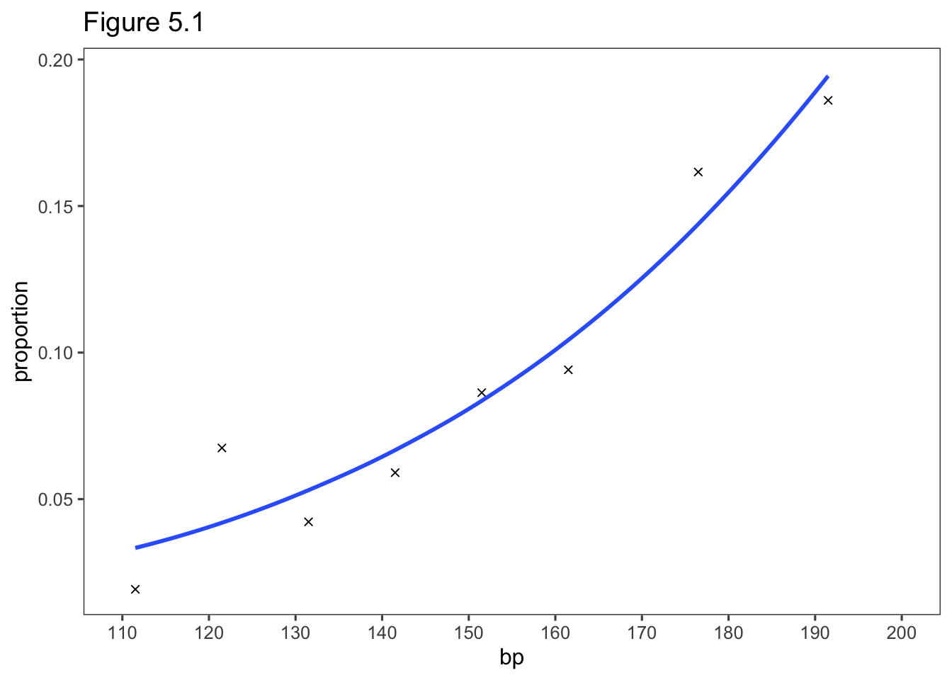
5.3 Infinite Estimates in Logistic Regression
5.3.1 Complete and Quasi-Complete Separation: Perfeect Discrination
library(tidyverse)
library(ggthemes)
data.frame (x = c(10, 20, 30, 40, 60, 70, 80, 90),
                         y = c(0, 0, 0, 0, 1, 1, 1, 1)) %>%
  ggplot(aes(x = x, y = y)) +
  geom_point() +
  theme_few() +
  ggtitle("Figure 5.2") +
  scale_y_continuous(breaks = c(0,1)) +
  theme(axis.text.x = element_blank(),
        axis.ticks.x = element_blank(),
        axis.title.y = element_text(angle = 0, vjust = 0.5),
plot.title = element_text(hjust = 0.5)) 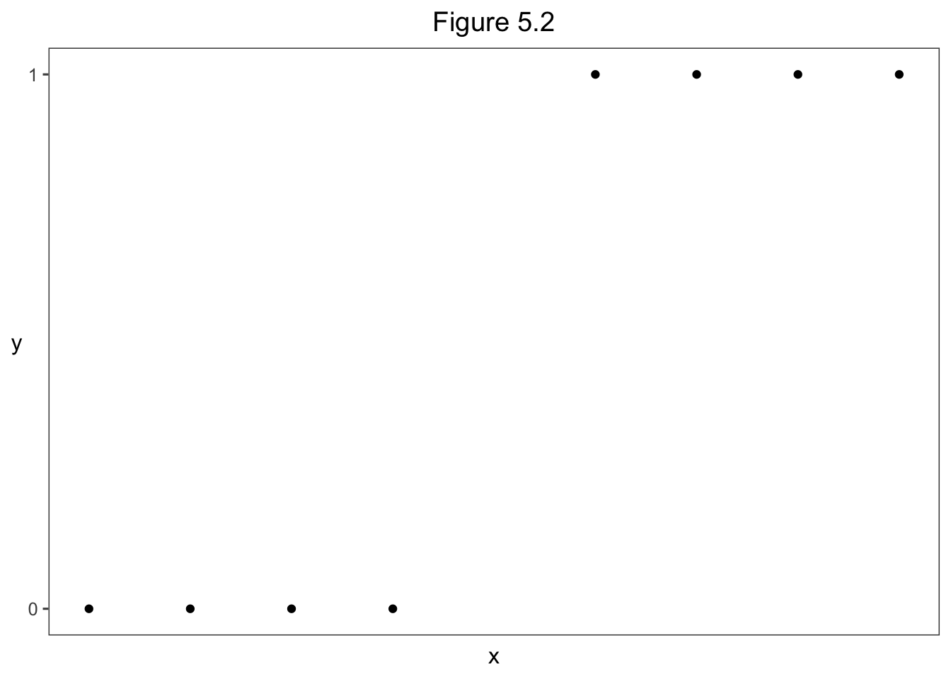
5.3.2 Example: Infinite Estimate for Toy Example
x <- c(10, 20, 30, 40, 60, 70, 80, 90)
y <- c(0, 0, 0, 0, 1, 1, 1, 1)

fit <- glm(y ~ x, family = binomial)
Warning: glm.fit: fitted probabilities numerically 0 or 1 occurred# P-value for Wald test of H0: beta = 0
# res deviance = 0 means perfect fit
# Fisher iterations: 25 shows very slow convergence
summary(fit)
Call:
glm(formula = y ~ x, family = binomial)

Deviance Residuals:
       Min          1Q      Median          3Q         Max
-1.045e-05  -2.110e-08   0.000e+00   2.110e-08   1.045e-05

Coefficients:
              Estimate Std. Error z value Pr(>|z|)
(Intercept)   -118.158 296046.187       0        1
x                2.363   5805.939       0        1

(Dispersion parameter for binomial family taken to be 1)

    Null deviance: 1.1090e+01  on 7  degrees of freedom
Residual deviance: 2.1827e-10  on 6  degrees of freedom
AIC: 4

Number of Fisher Scoring iterations: 25
# maximized log-likelihood = 0, so maximized likelihood = 1
logLik(fit)'log Lik.' -1.09134e-10 (df=2)#library(car)
# P-value for likelihood-ratio test of beta = 0 is more sensitive than p-value of 1 for Wald test
car::Anova(fit)Analysis of Deviance Table (Type II tests)
Response: y
LR Chisq Df Pr(>Chisq)
x 11.09 1 0.0008678 ***
---
Signif. codes: 0 '***' 0.001 '**' 0.01 '*' 0.05 '.' 0.1 ' ' 1library(profileModel) # ordinary confint function fails for infinite estimates
confintModel(fit, objective = "ordinaryDeviance", method = "zoom")Preliminary iteration .. Done
Profiling for parameter (Intercept) ... Done
Profiling for parameter x ... Done
Zooming for parameter (Intercept) ...
Zooming for parameter x ... Lower Upper
(Intercept) -Inf -2.66963
x 0.05876605 Inf
attr(,"fitted object")
fit5.3.4 Example: Risk Factors for Endometrial Cancer Grade
library(tidyverse)
Endo <- read.table("http://users.stat.ufl.edu/~aa/cat/data/Endometrial.dat",
                   header = TRUE, stringsAsFactors = TRUE)

Endo %>%
  filter(row_number() %in% c(1, 2, n()))
NV PI EH HG
1 0 13 1.64 0
2 0 16 2.26 0
3 0 33 0.85 1xtabs(~NV + HG, data = Endo) # quasi-complete separation when NV = 1, no HG=0 cases occur HG
NV 0 1
0 49 17
1 0 13fit <- glm(HG ~ NV + PI + EH, family = binomial, data = Endo)
# NV's true estimate is infinity
summary(fit)
Call:
glm(formula = HG ~ NV + PI + EH, family = binomial, data = Endo)

Deviance Residuals:
     Min        1Q    Median        3Q       Max
-1.50137  -0.64108  -0.29432   0.00016   2.72777

Coefficients:
              Estimate Std. Error z value Pr(>|z|)
(Intercept)    4.30452    1.63730   2.629 0.008563 **
NV            18.18556 1715.75089   0.011 0.991543
PI            -0.04218    0.04433  -0.952 0.341333
EH            -2.90261    0.84555  -3.433 0.000597 ***
---
Signif. codes:  0 '***' 0.001 '**' 0.01 '*' 0.05 '.' 0.1 ' ' 1

(Dispersion parameter for binomial family taken to be 1)

    Null deviance: 104.903  on 78  degrees of freedom
Residual deviance:  55.393  on 75  degrees of freedom
AIC: 63.393

Number of Fisher Scoring iterations: 17logLik(fit)'log Lik.' -27.69663 (df=4)library(car)
Anova(fit) # NV P= .0022 vs Wald 0.99Analysis of Deviance Table (Type II tests)
Response: HG
LR Chisq Df Pr(>Chisq)
NV 9.3576 1 0.002221 **
PI 0.9851 1 0.320934
EH 19.7606 1 8.777e-06 ***
---
Signif. codes: 0 '***' 0.001 '**' 0.01 '*' 0.05 '.' 0.1 ' ' 1library(profileModel) # ordinary confint function fails for infinite est
confintModel(fit, objective = "ordinaryDeviance", method = "zoom") # 95% profile likelihood CI for beta 1 Preliminary iteration .... Done
Profiling for parameter (Intercept) ... Done
Profiling for parameter NV ... Done
Profiling for parameter PI ... Done
Profiling for parameter EH ... Done
Zooming for parameter (Intercept) ...
Zooming for parameter NV ...
Zooming for parameter PI ...
Zooming for parameter EH ... Lower Upper
(Intercept) 1.4290183 7.94717425
NV 1.2856920 Inf
PI -0.1370717 0.03810556
EH -4.7866976 -1.43682244
attr(,"fitted object")
fitlibrary(detectseparation) # new package
# 0 denotes finite est, Inf denotes infinite est.
glm(HG ~ NV + PI + EH, family = binomial, data = Endo, method = "detectSeparation")Implementation: ROI | Solver: lpsolve
Separation: TRUE
Existence of maximum likelihood estimates
(Intercept) NV PI EH
0 Inf 0 0
0: finite value, Inf: infinity, -Inf: -infinity5.4 Bayesian Inference, Penalized Likelihood, and Conditional Likelihood for Logistic Regression *
5.4.2 Example: Risk Factors for Endometrial Caner Revisited
Endo2 <-
  Endo %>%
  mutate(PI2 = scale(PI),
         EH2 = scale(EH),
         NV2 = NV - 0.5)

fit.ML <- glm(HG ~ NV2 + PI2 + EH2, family = binomial, data = Endo2)
summary(fit.ML)
Call:
glm(formula = HG ~ NV2 + PI2 + EH2, family = binomial, data = Endo2)

Deviance Residuals:
     Min        1Q    Median        3Q       Max
-1.50137  -0.64108  -0.29432   0.00016   2.72777

Coefficients:
             Estimate Std. Error z value Pr(>|z|)
(Intercept)    7.8411   857.8755   0.009 0.992707
NV2           18.1856  1715.7509   0.011 0.991543
PI2           -0.4217     0.4432  -0.952 0.341333
EH2           -1.9219     0.5599  -3.433 0.000597 ***
---
Signif. codes:  0 '***' 0.001 '**' 0.01 '*' 0.05 '.' 0.1 ' ' 1

(Dispersion parameter for binomial family taken to be 1)

    Null deviance: 104.903  on 78  degrees of freedom
Residual deviance:  55.393  on 75  degrees of freedom
AIC: 63.393

Number of Fisher Scoring iterations: 17library(MCMCpack) # b0 = prior mean, B0 = prior precision = 1/varianceLoading required package: coda##
## Markov Chain Monte Carlo Package (MCMCpack)## Copyright (C) 2003-2023 Andrew D. Martin, Kevin M. Quinn, and Jong Hee Park##
## Support provided by the U.S. National Science Foundation## (Grants SES-0350646 and SES-0350613)
##fitBayes <- MCMClogit(HG ~ NV2 + PI2 + EH2, mcmc = 100000, b0 = 0, B0 = 0.01,
data = Endo2) # prior var = 1/0.01 = 100, sd = 10
summary(fitBayes) # posterior deviation
Iterations = 1001:101000
Thinning interval = 1
Number of chains = 1
Sample size per chain = 1e+05

1. Empirical mean and standard deviation for each variable,
   plus standard error of the mean:

               Mean     SD Naive SE Time-series SE
(Intercept)  3.2356 2.5948 0.008206       0.026682
NV2          9.1626 5.1639 0.016330       0.053109
PI2         -0.4711 0.4546 0.001437       0.006376
EH2         -2.1332 0.5879 0.001859       0.008450

2. Quantiles for each variable:

               2.5%     25%     50%     75%   97.5%
(Intercept) -0.3391  1.2619  2.7161  4.6972  9.4865
NV2          2.1105  5.2437  8.1064 12.1133 21.6077
PI2         -1.4163 -0.7676 -0.4445 -0.1538  0.3538
EH2 -3.3781 -2.5087 -2.0977 -1.7227 -1.0786mean(fitBayes[,2] < 0) # probability below 0 for 2n model parameter (NV2)[1] 0.000165.4.3 Penalized Likelihood Reduces Bias in Logistic Regression
\[L^*(\beta) = L(\beta) - s(\beta),\]
5.4.4 Example: Risk Factors for Endometrial Cancer Revisited
library(logistf)
fit.penalized <- logistf(HG ~ NV2 + PI2 + EH2, family=binomial, data=Endo2)
options(digits = 4)
summary(fit.penalized)
logistf(formula = HG ~ NV2 + PI2 + EH2, data = Endo2, family = binomial)
Model fitted by Penalized ML
Coefficients:
coef se(coef) lower 0.95 upper 0.95 Chisq p method
(Intercept) 0.3080 0.7585 -0.9755 2.7888 0.1690 6.810e-01 2
NV2 2.9293 1.4650 0.6097 7.8546 6.7985 9.124e-03 2
PI2 -0.3474 0.3788 -1.2443 0.4045 0.7468 3.875e-01 2
EH2 -1.7243 0.4990 -2.8903 -0.8162 17.7593 2.507e-05 2
Method: 1-Wald, 2-Profile penalized log-likelihood, 3-None
Likelihood ratio test=43.66 on 3 df, p=1.786e-09, n=79
Wald test = 21.67 on 3 df, p = 7.641e-05options(digits = 7)5.5 Alternative Link Functions: Linear Probability and Probit Models *
5.5.2 Example: Political Ideology and Belief in Evolution
library(tidyverse)
Evo <- read.table("http://users.stat.ufl.edu/~aa/cat/data/Evolution2.dat",
                        header = TRUE, stringsAsFactors = TRUE)

Evo %>%
  filter(row_number() %in% c(1, 2, n()))
ideology evolved
1 1 1
2 1 1
3 7 0fit <- glm(evolved ~ ideology,
family=quasi(link=identity, variance = "mu(1-mu)"),
data = Evo)
summary(fit, dispersion = 1)
Call:
glm(formula = evolved ~ ideology, family = quasi(link = identity,
    variance = "mu(1-mu)"), data = Evo)

Deviance Residuals:
    Min       1Q   Median       3Q      Max
-2.0558  -1.2617   0.7247   1.0954   1.7440

Coefficients:
            Estimate Std. Error z value Pr(>|z|)
(Intercept) 0.108437   0.038932   2.785  0.00535 **
ideology    0.110102   0.008971  12.273  < 2e-16 ***
---
Signif. codes:  0 '***' 0.001 '**' 0.01 '*' 0.05 '.' 0.1 ' ' 1

(Dispersion parameter for quasi family taken to be 1)

    Null deviance: 1469.3  on 1063  degrees of freedom
Residual deviance: 1359.5  on 1062  degrees of freedom
AIC: NA

Number of Fisher Scoring iterations: 3
fit2 <- glm(evolved ~ ideology, family=gaussian(link=identity), data = Evo)
summary(fit2)
Call:
glm(formula = evolved ~ ideology, family = gaussian(link = identity),
    data = Evo)

Deviance Residuals:
    Min       1Q   Median       3Q      Max
-0.8819  -0.5492   0.2290   0.4508   0.7836

Coefficients:
            Estimate Std. Error t value Pr(>|t|)
(Intercept)  0.10554    0.04272    2.47   0.0137 *
ideology     0.11091    0.01033   10.73   <2e-16 ***
---
Signif. codes:  0 '***' 0.001 '**' 0.01 '*' 0.05 '.' 0.1 ' ' 1

(Dispersion parameter for gaussian family taken to be 0.2247506)

    Null deviance: 264.57  on 1063  degrees of freedom
Residual deviance: 238.69  on 1062  degrees of freedom
AIC: 1435.2

Number of Fisher Scoring iterations: 2
5.5.3 Probit Model and Normal Latent Variable Model
\[\mathrm{probit}[F(Y = 1)] = \alpha + \beta_1 x_1 + \cdots + \beta_px_p\]
\[y^* = \alpha + \beta_1 x_1+ \cdots + \beta_px_p + \epsilon.\]
5.5.4 Example: Snoring and Heart Disease Revisited
\[\mathrm{probit}[\hat P(Y = 1)] = -2.061 + 0.188x.\]
library(tidyverse)
Heart <- read.table("http://users.stat.ufl.edu/~aa/cat/data/Heart.dat",
                        header = TRUE, stringsAsFactors = TRUE)
Heart
snoring yes no
1 never 24 1355
2 occasional 35 603
3 nearly_every_night 21 192
4 every_night 30 224# recode() is in dplyr and car...
Heart <- Heart %>%
mutate(snoringNights = dplyr::recode(snoring, never = 0, occasional = 2,
nearly_every_night = 4, every_night = 5))
fit <- glm(yes/(yes+no) ~ snoringNights, family = binomial(link = probit),
weights = yes+no, data = Heart)
summary(fit)
Call:
glm(formula = yes/(yes + no) ~ snoringNights, family = binomial(link = probit),
    data = Heart, weights = yes + no)

Deviance Residuals:
      1        2        3        4
-0.6188   1.0388   0.1684  -0.6175

Coefficients:
              Estimate Std. Error z value Pr(>|z|)
(Intercept)   -2.06055    0.07017 -29.367  < 2e-16 ***
snoringNights  0.18777    0.02348   7.997 1.28e-15 ***
---
Signif. codes:  0 '***' 0.001 '**' 0.01 '*' 0.05 '.' 0.1 ' ' 1

(Dispersion parameter for binomial family taken to be 1)

    Null deviance: 65.9045  on 3  degrees of freedom
Residual deviance:  1.8716  on 2  degrees of freedom
AIC: 26.124

Number of Fisher Scoring iterations: 4options(digits = 4)
fitted(fit) 1 2 3 4
0.01967 0.04599 0.09519 0.13100 options(digits = 7)