4 Logistic Regression
4.1 The Logistic Regression Model
4.1.1 The Logistic Regression Model
\[\begin{equation} \mathrm{logit}[\pi(x)] = \mathrm{log}\left[\frac{\pi(x)}{1=\pi(x)}\right]= \alpha + \beta x. \tag{6} \end{equation}\]
\[\begin{equation} \pi(x) = \frac{e^{\alpha + \beta x}}{1+e^{\alpha + \beta x}}. \tag{7} \end{equation}\]
4.1.2 Odds Ratio and Linear Approximaiton Interpreetations
\[\frac{\pi(x)}{1-\pi(x)}=\mathrm{exp}(\alpha + \beta x) = e^\alpha(e^\beta)^x.\]
Crabs <- read.table("http://users.stat.ufl.edu/~aa/cat/data/Crabs.dat",
  header = TRUE
)
library(RColorBrewer)
colors <- brewer.pal(n = 4, name = "Dark2")

fit <- glm(y ~ width, family = binomial, data = Crabs)
summary(fit)
Call:
glm(formula = y ~ width, family = binomial, data = Crabs)

Deviance Residuals:
    Min       1Q   Median       3Q      Max
-2.0281  -1.0458   0.5480   0.9066   1.6942

Coefficients:
            Estimate Std. Error z value Pr(>|z|)
(Intercept) -12.3508     2.6287  -4.698 2.62e-06 ***
width         0.4972     0.1017   4.887 1.02e-06 ***
---
Signif. codes:  0 '***' 0.001 '**' 0.01 '*' 0.05 '.' 0.1 ' ' 1

(Dispersion parameter for binomial family taken to be 1)

    Null deviance: 225.76  on 172  degrees of freedom
Residual deviance: 194.45  on 171  degrees of freedom
AIC: 198.45

Number of Fisher Scoring iterations: 4
at28 <- predict(fit, data.frame(width = 28), type = "resp")
at29 <- predict(fit, data.frame(width = 29), type = "resp")
x <- seq(20, 34, by = .01)
df <- tibble(x = x) %>%
mutate(y = predict(fit, data.frame(width = x), type = "resp"))
spl <- smooth.spline(df$x, df$y, spar = 0.3)
newx <- seq(min(df$x), max(df$x), 0.1)
pred <- predict(spl, x = newx, deriv = 0)
# solve for tangent at a given x
newx <- 28
pred0 <- predict(spl, x = newx, deriv = 0)
pred1 <- predict(spl, x = newx, deriv = 1)
yint <- pred0$y - (pred1$y * newx)
xint <- -yint / pred1$y
tang <- tibble(x = df$x) %>%
mutate(y = yint + pred1$y * x) %>%
filter(x > 25.5 & x < 30.5)
library(ggthemes)
aLabel <- as.vector(expression(paste(beta, pi, "(1-", pi, ")")))
ggplot() +
geom_line(data = df, aes(x = x, y = y)) +
geom_line(data = tang, aes(x = x, y = y)) +
annotate(
geom = "segment", x = 28, y = at28, xend = 28, yend = at29,
color = colors[1]
) +
annotate(
geom = "segment", x = 28, y = at29, xend = 29, yend = at29,
color = colors[1]
) +
annotate(
geom = "text", x = 26.35, y = at28 + .02,
label = 'paste(beta, pi, "(1-" , pi, ")")', parse = TRUE,
hjust = "left",
color = colors[1]
) +
annotate(
geom = "text", x = 28.3, y = at29 + .03,
label = "1",
hjust = "left",
color = colors[1]
) +
theme_few() +
theme(axis.title.y = element_text(angle = 0, vjust = .5)) +
scale_x_continuous(breaks = seq(20, 34, by = 2)) +
scale_y_continuous(breaks = seq(0, 1, by = .2)) +
ggtitle("Figure 4.1") +
xlab("Width") +
ylab("Probability")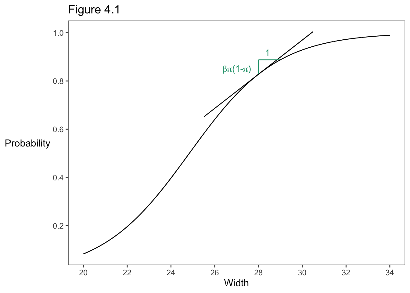
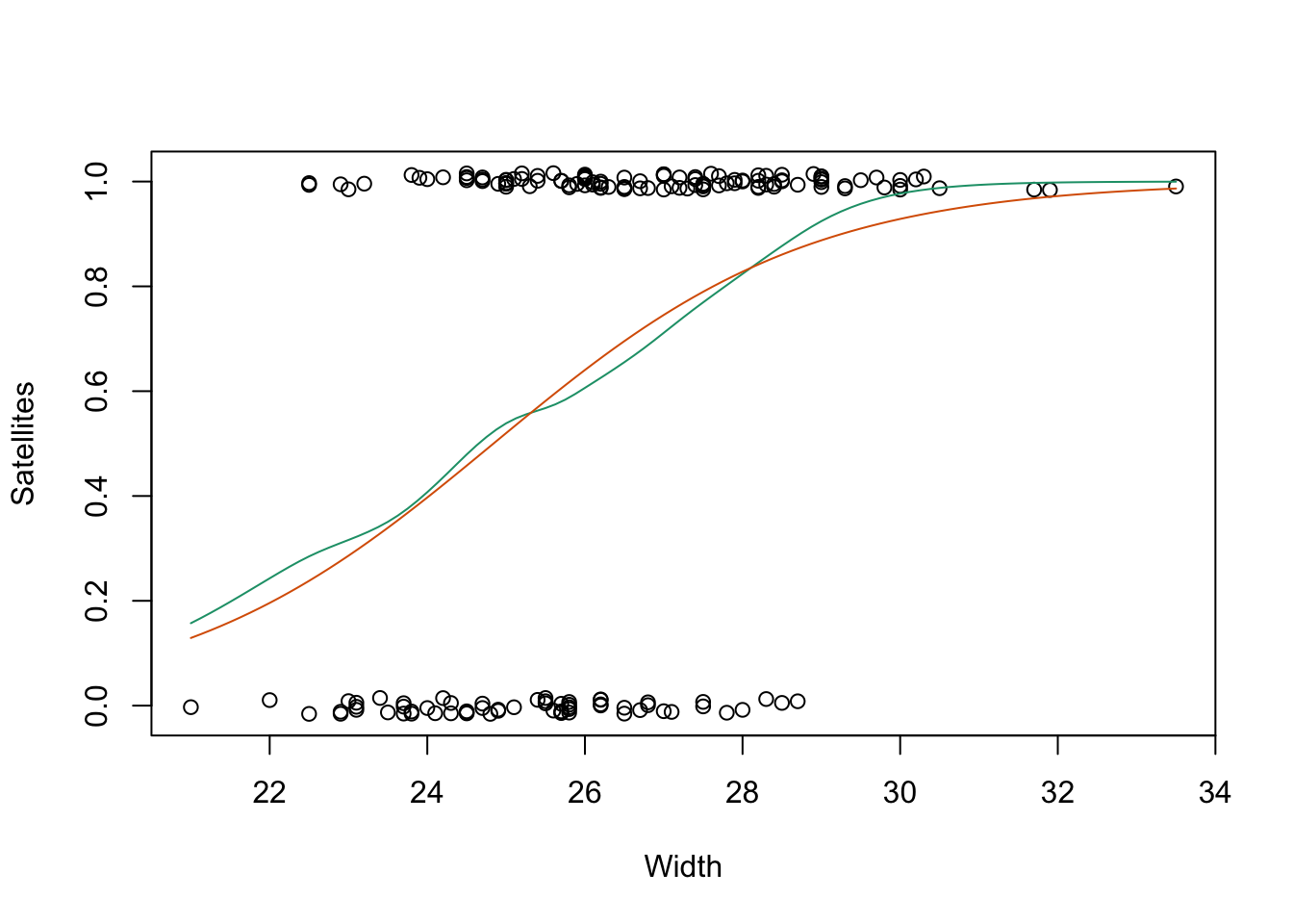
4.1.3 Example: Whethr a Female Horsehoe Crab Has Satelites
Crabs <- read.table("http://users.stat.ufl.edu/~aa/cat/data/Crabs.dat",
  header = TRUE
)

Crabs %>%
  filter(row_number() %in% c(1, 2, n()))
crab sat y weight width color spine
1 1 8 1 3.05 28.3 2 3
2 2 0 0 1.55 22.5 3 3
3 173 0 0 2.00 24.5 2 2library(RColorBrewer)
colors <- brewer.pal(n = 4, name = "Dark2")
library(gam)
gam.fit <- gam(y ~ s(width), family = binomial, data = Crabs)
fit <- glm(y ~ width, family = binomial, data = Crabs)
plot(jitter(y, 0.08) ~ width, data = Crabs, xlab = "Width", ylab = "Satellites")
curve(predict(gam.fit, data.frame(width = x), type = "resp"),
col = colors[1], add = TRUE
)
curve(predict(fit, data.frame(width = x), type = "resp"),
col = colors[2], add = TRUE
)
summary(fit)
Call:
glm(formula = y ~ width, family = binomial, data = Crabs)

Deviance Residuals:
    Min       1Q   Median       3Q      Max
-2.0281  -1.0458   0.5480   0.9066   1.6942

Coefficients:
            Estimate Std. Error z value Pr(>|z|)
(Intercept) -12.3508     2.6287  -4.698 2.62e-06 ***
width         0.4972     0.1017   4.887 1.02e-06 ***
---
Signif. codes:  0 '***' 0.001 '**' 0.01 '*' 0.05 '.' 0.1 ' ' 1

(Dispersion parameter for binomial family taken to be 1)

    Null deviance: 225.76  on 172  degrees of freedom
Residual deviance: 194.45  on 171  degrees of freedom
AIC: 198.45

Number of Fisher Scoring iterations: 4
# estimated probability of satellite at width = 21.0
predict(fit, data.frame(width = 21.0), type = "resp") 1
0.129096 predict(fit, data.frame(width = mean(Crabs$width)), type = "resp") 1
0.6738768 \[\mathrm{logit}[\hat\pi(x)] = -12.351 + 0.497 x.\]
\[\hat\pi(x) =\frac{\mathrm{exp}(-12.351 + 0.497 x)}{1+\mathrm{exp}(-12.351 + 0.497 x)}.\]
\[\frac{\mathrm{exp}[-12.351 + 0.497 (21.0)]}{1+\mathrm{exp}[-12.351 + 0.497 (21.0)]} = 0.129.\]
4.2 Statistical Inference for Logistic Regression
4.2.1 Confidence Intervals for Effects
Crabs <- read.table("http://users.stat.ufl.edu/~aa/cat/data/Crabs.dat",
  header = TRUE
)

fit <- glm(y ~ width, family = binomial, data = Crabs)
summary(fit) # z value & p-value Wald test
Call:
glm(formula = y ~ width, family = binomial, data = Crabs)

Deviance Residuals:
    Min       1Q   Median       3Q      Max
-2.0281  -1.0458   0.5480   0.9066   1.6942

Coefficients:
            Estimate Std. Error z value Pr(>|z|)
(Intercept) -12.3508     2.6287  -4.698 2.62e-06 ***
width         0.4972     0.1017   4.887 1.02e-06 ***
---
Signif. codes:  0 '***' 0.001 '**' 0.01 '*' 0.05 '.' 0.1 ' ' 1

(Dispersion parameter for binomial family taken to be 1)

    Null deviance: 225.76  on 172  degrees of freedom
Residual deviance: 194.45  on 171  degrees of freedom
AIC: 198.45

Number of Fisher Scoring iterations: 4suppressMessages(
confint(fit) # profile likelihood confidence interval
) 2.5 % 97.5 %
(Intercept) -17.8100090 -7.4572470
width 0.3083806 0.7090167suppressPackageStartupMessages(library(car))
Anova(fit) # likelihood-ratio test of width effectAnalysis of Deviance Table (Type II tests)
Response: y
LR Chisq Df Pr(>Chisq)
width 31.306 1 2.204e-08 ***
---
Signif. codes: 0 '***' 0.001 '**' 0.01 '*' 0.05 '.' 0.1 ' ' 14.2.3 Fitted Values and Confidence Intervals for Probabilities
\[\hat P(Y=1)=\mathrm{exp}(\hat\alpha + \hat\beta x)/[1 + (\hat\alpha + \hat\beta x)],\]
Crabs <- read.table("http://users.stat.ufl.edu/~aa/cat/data/Crabs.dat",
  header = TRUE, stringsAsFactors = TRUE
)

fit <- glm(y ~ width, family = binomial, data = Crabs)
pred.prob <- fitted(fit) # ML fitted value estimate of P(Y = 1)
lp <- predict(fit, se.fit = TRUE) # linear predictor
LB <- lp$fit - 1.96 * lp$se.fit # confidence bounds for linear predictor
LB <- lp$fit + qnorm(0.025) * lp$se.fit # better confidence bound
UB <- lp$fit + qnorm(0.975) * lp$se.fit
LB.p <- exp(LB) / (1 + exp(LB)) # confidence bounds for P(Y = 1)
UB.p <- exp(UB) / (1 + exp(UB))


library(dplyr) # bind_cols, filter, row_number
predictions <-
  bind_cols(
    Width = Crabs$width,
    `Predicted probaility` = pred.prob,
    `Lower CB` = LB.p,
    `Upper CB` = UB.p
  )

predictions %>%
  filter(row_number() %in% c(1, 7, n()))
# A tibble: 3 × 4
Width `Predicted probaility` `Lower CB` `Upper CB`
<dbl> <dbl> <dbl> <dbl>
1 28.3 0.848 0.753 0.911
2 26.5 0.695 0.612 0.768
3 24.5 0.458 0.356 0.564fit <- glm(y ~ width, family = binomial, data = Crabs)
library(tidyverse)
data.plot <- tibble(width = 18:34)
lp <- predict(fit, newdata = data.plot, se.fit = TRUE)
library(ggthemes)
data.plot <- data.plot %>%
mutate(
pred.prob = exp(lp$fit) / (1 + exp(lp$fit)),
LB = lp$fit + qnorm(0.025) * lp$se.fit,
UB = lp$fit + qnorm(0.975) * lp$se.fit,
LB.p = exp(LB) / (1 + exp(LB)),
UB.p = exp(UB) / (1 + exp(UB))
)
data.plot %>%
ggplot(aes(x = width)) +
geom_point(data = Crabs, aes(x = width, y = jitter(y, .1))) +
geom_line(aes(y = pred.prob)) +
geom_ribbon(aes(ymin = LB.p, ymax = UB.p), fill = "gray", alpha = 0.5) +
theme_few() +
ylab("Probability (satellites)") +
scale_y_continuous(breaks = seq(0, 1, by = .2)) +
xlab("Width") +
ggtitle("Figure 4.3")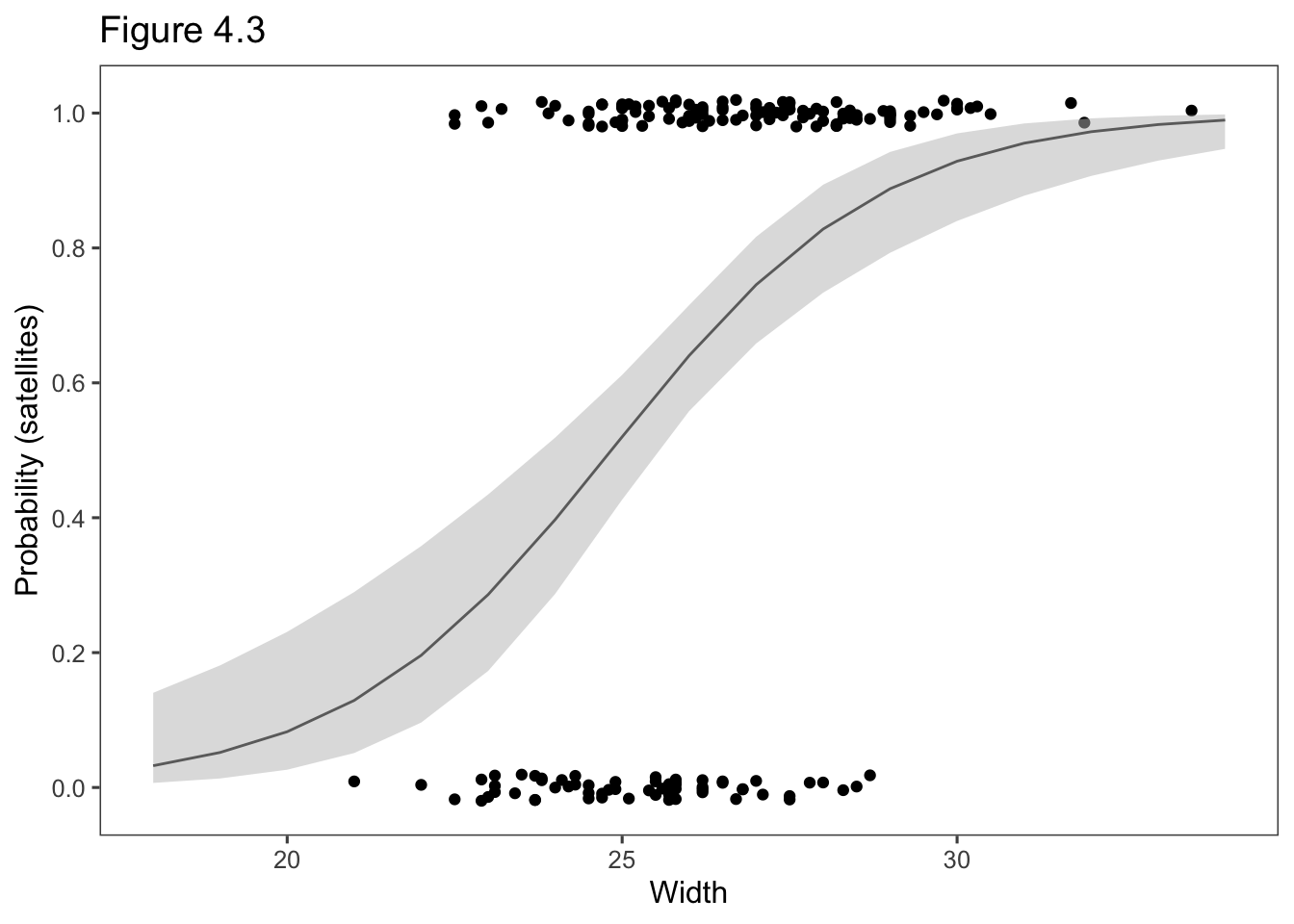
4.3 Logistic Regression with Categorical Predictors
4.3.1 Indicator Variables Represent Categories of Predictors
\[\mathrm{logit}[P(Y = 1)] = \alpha + \beta_1 x + \beta_2 z\]
| x | z | Logit |
|---|---|---|
| 0 | 0 | \(\alpha\) |
| 1 | 0 | \(\alpha + \beta_1\) |
| 0 | 0 | \(\alpha + \beta_2\) |
| 0 | 0 | \(\alpha + \beta_1 + \beta_2\) |
\[ = [\alpha + \beta_1 (1) + \beta_2 z] - [\alpha + \beta_1 (0) + \beta_2 z] = \beta_a.\]
4.3.2 Example: Survey about Marijuana Use
library(tidyverse)
Marijuana <- read.table("http://users.stat.ufl.edu/~aa/cat/data/Marijuana.dat",
  header = TRUE, stringsAsFactors = TRUE
)

Marijuana
race gender yes no
1 white female 420 620
2 white male 483 579
3 other female 25 55
4 other male 32 62fit <- glm(yes / (yes + no) ~ gender + race,
weights = yes + no, family = binomial,
data = Marijuana
)
theFit <- summary(fit)
theFit
Call:
glm(formula = yes/(yes + no) ~ gender + race, family = binomial,
    data = Marijuana, weights = yes + no)

Deviance Residuals:
       1         2         3         4
-0.04513   0.04402   0.17321  -0.15493

Coefficients:
            Estimate Std. Error z value Pr(>|z|)
(Intercept) -0.83035    0.16854  -4.927 8.37e-07 ***
gendermale   0.20261    0.08519   2.378  0.01739 *
racewhite    0.44374    0.16766   2.647  0.00813 **
---
Signif. codes:  0 '***' 0.001 '**' 0.01 '*' 0.05 '.' 0.1 ' ' 1

(Dispersion parameter for binomial family taken to be 1)

    Null deviance: 12.752784  on 3  degrees of freedom
Residual deviance:  0.057982  on 1  degrees of freedom
AIC: 30.414

Number of Fisher Scoring iterations: 3
# pull the 2nd and 3rd element from the "Estimate" column, exponentiate & round
round(exp(theFit$coefficients[2:3, "Estimate"]), 2)gendermale racewhite
1.22 1.56 # easier to follow syntax
theCoef <- as.data.frame(coef(theFit))
theCoef %>%
rownames_to_column(var = "Effect") %>%
select("Effect", "Estimate") %>%
filter(Effect != "(Intercept)") %>%
mutate(`Odds Ratio` = exp(Estimate)) %>%
mutate_if(is.numeric, round, digits = 2) Effect Estimate Odds Ratio
1 gendermale 0.20 1.22
2 racewhite 0.44 1.56# library(car)
car::Anova(fit) # likelihood-ratio test for individual explanatory variablesAnalysis of Deviance Table (Type II tests)
Response: yes/(yes + no)
LR Chisq Df Pr(>Chisq)
gender 5.6662 1 0.017295 *
race 7.2770 1 0.006984 **
---
Signif. codes: 0 '***' 0.001 '**' 0.01 '*' 0.05 '.' 0.1 ' ' 14.4 Multiple Logistic Regression
\[\mathrm{logit}[P(Y=1)] = \alpha + \beta_1 x_1 + \beta_2 x_2 + \cdots + \beta_p x_p.\]
4.4.1 Example: Horseshoe Crabs with Color and Width Predictors
\[\begin{equation} \mathrm{logit}[P(Y=1)] = \alpha + \beta_1 x + \beta_2 c_2 + \beta_3 c_3 + \beta_4 c_4. \tag{8} \end{equation}\]
Crabs <- read.table("http://users.stat.ufl.edu/~aa/cat/data/Crabs.dat",
  header = TRUE, stringsAsFactors = TRUE
)

fit <- glm(y ~ width + factor(color), family = binomial, data = Crabs)
summary(fit)
Call:
glm(formula = y ~ width + factor(color), family = binomial, data = Crabs)

Deviance Residuals:
    Min       1Q   Median       3Q      Max
-2.1124  -0.9848   0.5243   0.8513   2.1413

Coefficients:
                Estimate Std. Error z value Pr(>|z|)
(Intercept)    -11.38519    2.87346  -3.962 7.43e-05 ***
width            0.46796    0.10554   4.434 9.26e-06 ***
factor(color)2   0.07242    0.73989   0.098    0.922
factor(color)3  -0.22380    0.77708  -0.288    0.773
factor(color)4  -1.32992    0.85252  -1.560    0.119
---
Signif. codes:  0 '***' 0.001 '**' 0.01 '*' 0.05 '.' 0.1 ' ' 1

(Dispersion parameter for binomial family taken to be 1)

    Null deviance: 225.76  on 172  degrees of freedom
Residual deviance: 187.46  on 168  degrees of freedom
AIC: 197.46

Number of Fisher Scoring iterations: 4
\[\mathrm{exp}[12.715 + 0.468(26.3)]/\{1 + \mathrm{exp}[12.715 + 0.468(26.3)]\}=0.399.\]
\[\mathrm{exp}[11.385 + 0.468(26.3)]/\{1 + \mathrm{exp}[11.385 + 0.468(26.3)]\} = 0.715.\]
4.4.2 Model Comparison to Check Whether a Term is Needed
summary(glm(y ~ width, family = binomial, data = Crabs))
Call:
glm(formula = y ~ width, family = binomial, data = Crabs)

Deviance Residuals:
    Min       1Q   Median       3Q      Max
-2.0281  -1.0458   0.5480   0.9066   1.6942

Coefficients:
            Estimate Std. Error z value Pr(>|z|)
(Intercept) -12.3508     2.6287  -4.698 2.62e-06 ***
width         0.4972     0.1017   4.887 1.02e-06 ***
---
Signif. codes:  0 '***' 0.001 '**' 0.01 '*' 0.05 '.' 0.1 ' ' 1

(Dispersion parameter for binomial family taken to be 1)

    Null deviance: 225.76  on 172  degrees of freedom
Residual deviance: 194.45  on 171  degrees of freedom
AIC: 198.45

Number of Fisher Scoring iterations: 4
# compare deviance = 194.45 vs 187.46 with color also in model
library(car)
Anova(glm(y ~ width + factor(color), family = binomial, data = Crabs))Analysis of Deviance Table (Type II tests)
Response: y
LR Chisq Df Pr(>Chisq)
width 24.6038 1 7.041e-07 ***
factor(color) 6.9956 3 0.07204 .
---
Signif. codes: 0 '***' 0.001 '**' 0.01 '*' 0.05 '.' 0.1 ' ' 14.4.3 Example: Treating Color as Quantitative or Binary
\[\begin{equation} \mathrm{logit}[P(Y=1)] = \alpha + \beta_1 x + \beta_2 c. \tag{9} \end{equation}\]
fit2 <- (glm(y ~ width + color, family = binomial, data = Crabs))
summary(fit2)
Call:
glm(formula = y ~ width + color, family = binomial, data = Crabs)

Deviance Residuals:
    Min       1Q   Median       3Q      Max
-2.1692  -0.9889   0.5429   0.8700   1.9742

Coefficients:
            Estimate Std. Error z value Pr(>|z|)
(Intercept) -10.0708     2.8068  -3.588 0.000333 ***
width         0.4583     0.1040   4.406 1.05e-05 ***
color        -0.5090     0.2237  -2.276 0.022860 *
---
Signif. codes:  0 '***' 0.001 '**' 0.01 '*' 0.05 '.' 0.1 ' ' 1

(Dispersion parameter for binomial family taken to be 1)

    Null deviance: 225.76  on 172  degrees of freedom
Residual deviance: 189.12  on 170  degrees of freedom
AIC: 195.12

Number of Fisher Scoring iterations: 4anova(fit2, fit, test = "LRT") # likelihood-ratio test comparing modelsAnalysis of Deviance Table
Model 1: y ~ width + color
Model 2: y ~ width + factor(color)
Resid. Df Resid. Dev Df Deviance Pr(>Chi)
1 170 189.12
2 168 187.46 2 1.6641 0.4351Crabs$c4 <- ifelse(Crabs$color == 4, 1, 0)
# Crabs$c4 <- I(Crabs$color == 4)
fit3 <- glm(y ~ width + c4, family = binomial, data = Crabs)
summary(fit3)
Call:
glm(formula = y ~ width + c4, family = binomial, data = Crabs)

Deviance Residuals:
    Min       1Q   Median       3Q      Max
-2.0821  -0.9932   0.5274   0.8606   2.1553

Coefficients:
            Estimate Std. Error z value Pr(>|z|)
(Intercept) -11.6790     2.6925  -4.338 1.44e-05 ***
width         0.4782     0.1041   4.592 4.39e-06 ***
c4           -1.3005     0.5259  -2.473   0.0134 *
---
Signif. codes:  0 '***' 0.001 '**' 0.01 '*' 0.05 '.' 0.1 ' ' 1

(Dispersion parameter for binomial family taken to be 1)

    Null deviance: 225.76  on 172  degrees of freedom
Residual deviance: 187.96  on 170  degrees of freedom
AIC: 193.96

Number of Fisher Scoring iterations: 4anova(fit3, fit, test = "LRT")Analysis of Deviance Table
Model 1: y ~ width + c4
Model 2: y ~ width + factor(color)
Resid. Df Resid. Dev Df Deviance Pr(>Chi)
1 170 187.96
2 168 187.46 2 0.50085 0.77854.4.4 Allowing Interaction between Explanatory Variables
(interaction <- glm(y ~ width + c4 + width:c4, family = binomial, data = Crabs))
Call:  glm(formula = y ~ width + c4 + width:c4, family = binomial, data = Crabs)

Coefficients:
(Intercept)        width           c4     width:c4
   -12.8117       0.5222       6.9578      -0.3217

Degrees of Freedom: 172 Total (i.e. Null);  169 Residual
Null Deviance:      225.8
Residual Deviance: 186.8 AIC: 194.8summary(interaction)
Call:
glm(formula = y ~ width + c4 + width:c4, family = binomial, data = Crabs)

Deviance Residuals:
    Min       1Q   Median       3Q      Max
-2.1366  -0.9344   0.4996   0.8554   1.7753

Coefficients:
            Estimate Std. Error z value Pr(>|z|)
(Intercept) -12.8117     2.9576  -4.332 1.48e-05 ***
width         0.5222     0.1146   4.556 5.21e-06 ***
c4            6.9578     7.3182   0.951    0.342
width:c4     -0.3217     0.2857  -1.126    0.260
---
Signif. codes:  0 '***' 0.001 '**' 0.01 '*' 0.05 '.' 0.1 ' ' 1

(Dispersion parameter for binomial family taken to be 1)

    Null deviance: 225.76  on 172  degrees of freedom
Residual deviance: 186.79  on 169  degrees of freedom
AIC: 194.79

Number of Fisher Scoring iterations: 4
# P-value 0.28 from last paragraph of 4.4.4
car::Anova(interaction)Analysis of Deviance Table (Type II tests)
Response: y
LR Chisq Df Pr(>Chisq)
width 26.8351 1 2.216e-07 ***
c4 6.4948 1 0.01082 *
width:c4 1.1715 1 0.27909
---
Signif. codes: 0 '***' 0.001 '**' 0.01 '*' 0.05 '.' 0.1 ' ' 14.5 Summarizing Effects in Logistic Regression
4.5.1 Probability-Based Interpretations
fit3 <- glm(y ~ width + c4, family = binomial, data = Crabs)

round(
  predict(fit3,
    data.frame(c4 = 1, width = mean(Crabs$width)),
    type = "response"
  ),
  3
)
1
0.401 round(
predict(fit3,
data.frame(c4 = 0, width = mean(Crabs$width)),
type = "response"
),
3
) 1
0.71 round(
predict(fit3, data.frame(c4 = mean(Crabs$c4), width = quantile(Crabs$width)),
type = "response"
),
3
) 0% 25% 50% 75% 100%
0.142 0.516 0.654 0.803 0.985 4.5.2 Marginal Effects and Their Average
fit3 <- glm(y ~ width + c4, family = binomial, data = Crabs)

suppressPackageStartupMessages(library(mfx))

# with atmean = TRUE, finds effect only at the mean
logitmfx(fit3, atmean = FALSE, data = Crabs)
Call:
logitmfx(formula = fit3, data = Crabs, atmean = FALSE)
Marginal Effects:
dF/dx Std. Err. z P>|z|
width 0.087483 0.024472 3.5748 0.0003504 ***
c4 -0.261420 0.105690 -2.4735 0.0133809 *
---
Signif. codes: 0 '***' 0.001 '**' 0.01 '*' 0.05 '.' 0.1 ' ' 1
dF/dx is for discrete change for the following variables:
[1] "c4"4.6 Summzarizing Predictive Power: Classification Tables, ROC Curves and Multiple Correlation
4.6.1 Summarizing Predictive Power: Classification Tables
Crabs <- read.table("http://users.stat.ufl.edu/~aa/cat/data/Crabs.dat",
  header = TRUE, stringsAsFactors = TRUE
)

prop <- sum(Crabs$y) / nrow(Crabs)
prop
[1] 0.6416185fit <- glm(y ~ width + factor(color), family = binomial, data = Crabs)
predicted <- as.numeric(fitted(fit) > prop) # predict y=1 when est. > 0.6416
xtabs(~ Crabs$y + predicted) predicted
Crabs$y 0 1
0 43 19
1 36 75# Make Table 4.4
predicted50 <- as.numeric(fitted(fit) > 0.50) # predict y=1 when est. > 0.50
xtabs(~ Crabs$y + predicted50) predicted50
Crabs$y 0 1
0 31 31
1 15 96# reorder levels to flip rows and columns
t1 <- xtabs(~ relevel(as.factor(Crabs$y), "1") + relevel(as.factor(predicted), "1"))
t1df <- as.data.frame.matrix(t1) %>%
rename("t1_1" = `1`) %>%
rename("t1_0" = `0`)
t2 <- xtabs(~ relevel(as.factor(Crabs$y), "1") + relevel(as.factor(predicted50), "1"))
t2df <- as.data.frame.matrix(t2) %>%
rename("t2_1" = `1`) %>%
rename("t2_0" = `0`)
Actual <-tibble(Actual = c("y = 1", "y = 0"))
Total <- tibble(Total = c(111, 62))
library(officer) # for fp_border() this needs to load before flextable
library(flextable)
suppressMessages(conflict_prefer("compose", "flextable"))
library(dplyr) # for bind_cols()
# Make analysis table
`Table 4.4` <- bind_cols(Actual, t1df, t2df, Total)
# The header needs blank columns for spaces in actual table.
# The wide column labels use Unicode characters for pi. Those details are
# replaced later with the compose() function.
theHeader <- data.frame(
col_keys = c("Actual", "blank", "t1_1", "t1_0",
"blank2", "t2_1", "t2_0",
"blank3", "Total"),
line1 = c("Actual", "",
rep("Prediction, \U1D70B = 0.6416", 2), "",
rep("Prediction, \U1D70B = 0.50", 2), "",
"Total"),
line2 = c("Actual", "", "t1_1", "t1_0", "", "t2_1", "t2_0", "", "Total"))
# Border lines
big_border <- fp_border(color="black", width = 2)
# Make the table - compose uses Unicode character
# https://stackoverflow.com/questions/64088118/in-r-flextable-can-complex-symbols-appear-in-column-headings
flextable(`Table 4.4`, col_keys = theHeader$col_keys) %>%
set_header_df(mapping = theHeader, key = "col_keys") %>%
theme_booktabs() %>%
merge_v(part = "header") %>%
merge_h(part = "header") %>%
align(align = "center", part = "all") %>%
empty_blanks() %>%
fix_border_issues() %>%
set_caption(caption = "Classification tables for horseshoe crab data with width and factor color predictors.") %>%
set_table_properties(width = 1, layout = "autofit") %>%
hline_top(part="header", border = big_border) %>%
hline_bottom(part="body", border = big_border) %>%
# i = 1 refers to top row of column headerings
compose(i = 1, j = "t1_1", part = "header",
value = as_paragraph("Prediction, \U1D70B",
as_sub("0"), "= 0.6416")) %>%
compose(i = 1, j = "t2_1", part = "header",
value = as_paragraph("Prediction, \U1D70B",
as_sub("0"), "= 0.50")) %>%
# i = 2 refers to second row of column headings
compose(part = "header", i = 2, j = "t1_1",
value = as_paragraph("y\U0302 = 1")) %>%
compose(part = "header", i = 2, j = "t1_0",
value = as_paragraph("y\U0302 = 0")) %>%
compose(part = "header", i = 2, j = "t2_1",
value = as_paragraph("y\U0302 = 1")) %>%
compose(part = "header", i = 2, j = "t2_0",
value = as_paragraph("y\U0302 = 0"))Actual | Prediction, 𝜋0= 0.6416 | Prediction, 𝜋0= 0.50 | Total | |||||
|---|---|---|---|---|---|---|---|---|
ŷ = 1 | ŷ = 0 | ŷ = 1 | ŷ = 0 | |||||
y = 1 | 75 | 36 | 96 | 15 | 111 | |||
y = 0 | 19 | 43 | 31 | 31 | 62 | |||
\[\mathrm{Sensitivity} = P(\hat y = 1 | y = 1), \ \ \ \ \ \mathrm{Sensitivity} = P(\hat y = 0 | y = 0)\]
\[P(\mathrm{correct\ classif.}) = \mathrm{sensitivity}[P(y = 1)] + \mathrm{specificity}[1 - P(y = 1)],\]
4.6.2 Summarizing Predictive Power: ROC Curves
fit <- glm(y ~ width + factor(color), family = binomial, data = Crabs)

suppressMessages(library(pROC))
suppressMessages(
  rocPlot <- roc(y ~ fitted(fit), data = Crabs)
)

x <- data.frame(rocPlot$sensitivities,rocPlot$specificities, rocPlot$thresholds)

thePar <- par(pty = "s")
plot.roc(rocPlot, legacy.axes = TRUE, asp = F)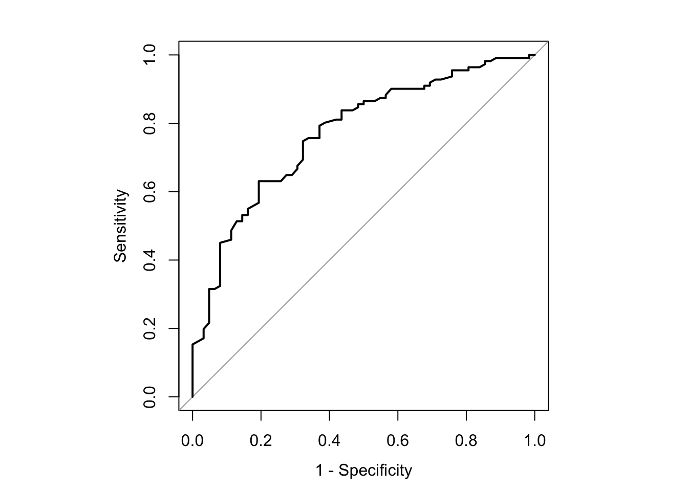
par(thePar)

auc(rocPlot)
Area under the curve: 0.7714# Make a prettier ROC plot including the probability cut points
model <- data.frame(outcome = Crabs$y,
predicted = predict(fit, Crabs, type = "response"))
suppressMessages(library(plotROC))
# `d` (disease) holds the known truth
# `m` (marker) holds the predictor values
ggplot(model, aes(d = outcome, m = predicted)) +
geom_roc() +
style_roc(xlab = "1-Specificity",
ylab ="Sensitivity",
minor.breaks = c(seq(0, 0.1, by = 0.02), seq(0.9, 1, by = 0.02))) +
ggtitle("ROC curve with probabilty cutpoints") +
theme(aspect.ratio=1) +
geom_abline(slope = 1, color = "grey92")Warning: The following aesthetics were dropped during statistical transformation: d, m
ℹ This can happen when ggplot fails to infer the correct grouping structure in
the data.
ℹ Did you forget to specify a `group` aesthetic or to convert a numerical
variable into a factor?